The Old Guard: How Traditional ML Conquered Tabular Data (Part 2 of 5)

The Reigning Champions

If you've ever applied for a credit card, had your insurance premium calculated, or seen a "customers also bought" recommendation, you've been touched by gradient boosted decision trees. These algorithms—with names like XGBoost, LightGBM, and CatBoost—have been the undisputed rulers of tabular machine learning for over a decade.

And here's the thing: they're really, really good at what they do.

Before we get into the advantages of tabular foundation models, let's understand why these traditional methods have worked so well.

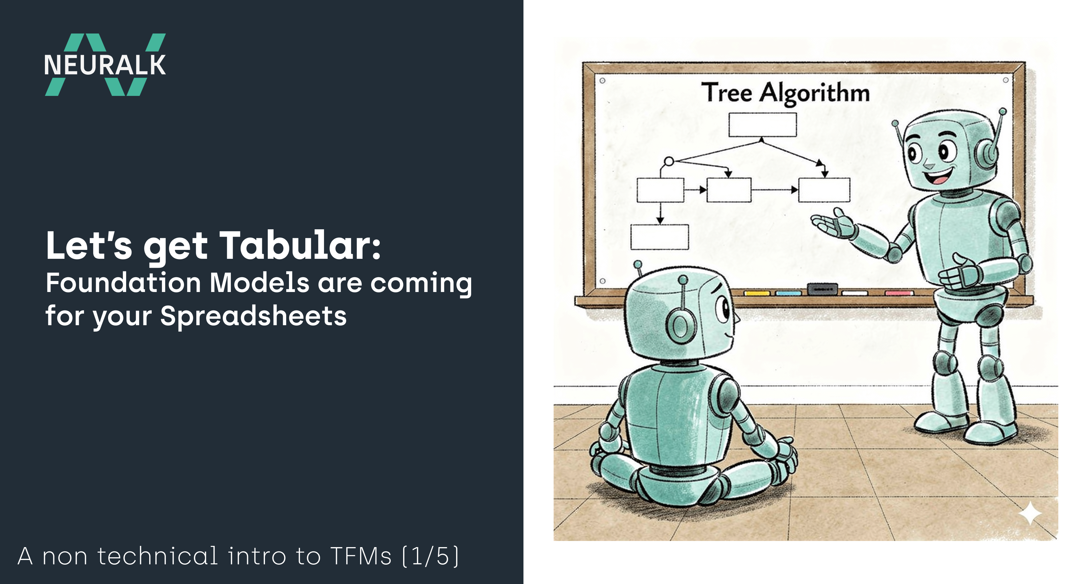
Decision Trees: Where It All Starts

Every tree-based algorithm starts with the humble decision tree—one of the most intuitive concepts in machine learning.

Imagine you're trying to predict whether a loan applicant will default. A decision tree might work like this:

1. Is their annual income above $50,000? If yes, go left. If no, go right.
2. On the left branch: Is their credit score above 700? If yes, predict "won't default." If no, keep splitting.
3. On the right branch: Do they have more than 3 existing loans? If yes, predict "will default". If no, keep splitting.

This continues until the tree reaches a prediction for every possible combination of features. Each path through the tree represents a simple rule: "IF income > $50k AND credit_score > 700 AND existing_loans < 3 THEN low_risk."

The beauty of decision trees is transparency. You can literally draw the decision process and explain it to anyone. The problem? A single tree is either too simple to capture complex patterns, or prone to overfitting—memorizing the training data rather than learning generalizable patterns.

‍

Random Forests: The Wisdom of Crowds

The solution to a single weak tree? Build hundreds of them.

Random Forest (introduced by Leo Breiman in 2001) creates many decision trees, each trained on a random subset of your data and using a random subset of your features. When it's time to make a prediction, every tree ‘votes’, and the majority wins.

Why does this work? Each individual tree might make mistakes, but they'll make different mistakes. By averaging across hundreds of diverse trees, the random errors cancel out, leaving you with a more robust prediction. It's the same principle behind asking a crowd to guess the number of jellybeans in a jar—individual guesses vary wildly, but the average is often eerily accurate.

The term for this is ensemble learning, and more specifically ensemble bagging: combining multiple weak learners into one strong learner.

Gradient Boosting: Learning from Mistakes

Random Forests build trees in parallel—each tree is independent. Gradient Boosting takes a different approach: it builds trees sequentially, with each new tree specifically trying to correct the mistakes of the previous ones.

Here's the intuition:

1. Build a simple tree. Make predictions. Calculate the errors.
2. Build a second tree, but instead of predicting the original target, train it to predict the errors from step 1.
3. Combine the predictions: original tree + error-correcting tree.
4. Calculate the remaining errors. Build a third tree to predict those errors.
5. Repeat for hundreds of iterations.

Each tree is small and weak on its own, but together they form a powerful predictive system. The "gradient" part refers to using calculus (specifically, gradients) to figure out exactly how each tree should correct the previous ensemble's mistakes.

XGBoost (2016), LightGBM (2017), and CatBoost (2017) are all implementations of gradient boosting with various optimizations for speed, memory efficiency, and handling of categorical variables.

The Linear Baseline: Logistic Regression

Not everything needs to be a tree. Logistic regression—despite its name, it's used for classification—remains a staple for tabular problems.

Logistic regression finds the best linear combination of your features that separates classes. If you have features like income, age, and credit score, it learns weights:

Prediction = w1*income + w2*age + w3*credit_score + bias


The prediction is then passed through a sigmoid function to produce a probability between 0 and 1.

Why use something so simple when you have XGBoost? Three reasons:

1. Interpretability: The weights directly tell you feature importance. A weight of 0.5 on income and -0.2 on age is immediately understandable.
2. Regulatory compliance: In industries like finance and healthcare, you often need to document and explain why a model made a decision. Linear models make this easy.
3. When it works, it works: If the true relationship in your data is approximately linear, why bring a cannon to a knife fight?

‍

The Traditional ML Workflow

So how do data scientists actually use these tools? Here's the typical workflow:

1. Data Collection & Exploration

Gather your data. Look at distributions, missing values, outliers. Understand what you're working with.

2. Train/Test Split

This is crucial. You split your data into two parts:

• Training set (~80%): The model learns from this data
• Test set (~20%): Held back to evaluate how well the model generalizes to new, unseen data

Why split? If you evaluate on the same data you trained on, you're just testing the model's memory, not its understanding. A student who memorizes the textbook will ace questions from the book but fail when asked something slightly different. The test set is your final exam with questions the model has never seen.

In practice, data scientists design several splits onto which the model can be evaluated to make sure the trained model is really robust and that the performance is actually statistically significant; but for the sake of keeping the explanation simple, we will keep a 1-fold evaluation process.

3. Feature Engineering and Preprocessing

This is where the magic (and suffering) happens. Raw data rarely feeds directly into models. You might:

• Create or select new features: ratio of debt to income, days since last purchase;
• Encode categorical variables: convert "red" / "green" / "blue" to numbers
• Handle missing values: fill with median, use a flag, or let the model handle it
• Normalize/scale: ensure features are on comparable scales

This step often determines success or failure. Domain expertise matters enormously.

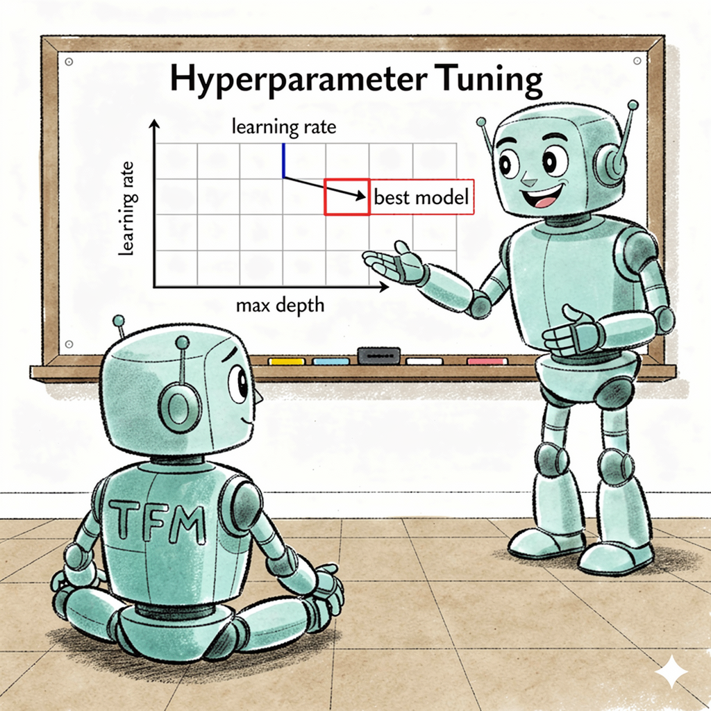
4. Model Selection & Hyperparameter Tuning

Choose your algorithm (random forest, XGBoost, logistic regression).

Models have settings that aren't learned from data:

• How deep should trees grow?
• How many trees to build?
• What learning rate to use?

Finding the best settings requires trying many combinations, typically using cross-validation: repeatedly splitting the training data into sub-folds, training on some and validating on others, to estimate how well each setting will generalize.

This step is time-consuming. Tuning XGBoost properly can take hours or days.

5. Model training

Train your model on the training set. The model adjusts its internal parameters to minimize prediction errors.

6. Evaluation

Finally, evaluate on the held-out test set. Common metrics include:

• Accuracy: What percentage of predictions are correct?
• AUC-ROC: How well does the model rank positive examples above negative ones?
• Precision/Recall: For imbalanced classes, how many predicted positives are true positives? How many true positives did we find?

1. Check feature contributions

This step is used to check whether there is any bias in the model decision. We can use feature importance scores or partial dependence plots to understand which features drive predictions, and look for unexpected patterns. Validate that decisions align with domain knowledge and fairness requirements.

Why Trees Dominate Tabular Data

Deep learning conquered images, text, and speech. Why not tables?

Several reasons:

1. Tabular data is fundamentally different

In an image, neighboring pixels have meaning—they form edges, textures, objects. In text, word order matters. But in a table, column order is arbitrary. Income next to age isn't meaningful the way a nose next to eyes is meaningful. Trees don't assume spatial relationships; they just find the best splits.

2. Trees handle heterogeneity naturally

Tabular data mixes numeric columns (income: 52,000), categorical columns (city: "London"), and ordinal columns (education: "high school" < "bachelor's" < "master's"). Trees handle all of these without special preprocessing. Neural networks struggle more.

3. Trees are robust to feature scale

A neural network cares whether income is measured in dollars (50,000) or millions (0.05). A tree doesn't—it just finds the split point. This reduces preprocessing burden.

4. Trees can capture non-linear interactions

The split "income > $50k" has different effects depending on other features. Trees naturally capture these interactions without explicitly programming them.

5. Trees are relatively fast

Training and inference are efficient, even for large datasets.

The Limitations

Of course, traditional methods aren't perfect:

Small data struggles: With only a few hundred training examples, most classic ML models will overfit. There simply aren't enough patterns to learn from.

No transfer learning: Every new dataset starts from scratch. The model learns nothing from the millions of previous tabular problems solved by others.

Extensive tuning required: Getting the best performance requires significant hyperparameter tuning. This is where tabular foundation models have a clear advantage.

Calibration quantification: Trees give you point predictions. Getting well-calibrated probability estimates ("I'm 73% sure this customer will churn") requires additional work.

‍

‍

Setting the Stage for Tabular Fondation Models

Traditional ML methods earned their dominance. They're fast, interpretable (at least the simpler ones), robust to the quirks of tabular data, and battle-tested across industries.

But they share a fundamental limitation: each model is trained from scratch on each new dataset. The knowledge gained from solving one tabular problem doesn't transfer to the next; there have been attempts in the past several years, but none have succeeded.

This is exactly what tabular foundation models aim to change. By pre-training on millions of diverse tables, they arrive at your dataset with prior knowledge—patterns already learned, statistical intuitions already formed.

The next article explores how you train a model on millions of tables when clean, labeled tabular data is actually quite rare. The answer involves a surprising amount of fake data.

Key Takeaways

→ Decision trees split data using simple rules; they're intuitive but prone to overfitting

→ Random Forests combine hundreds of trees trained on random subsets—errors cancel out

→ Gradient Boosting builds trees sequentially, each correcting the previous ensemble's mistakes

→ The traditional workflow involves train/test splits, feature engineering, hyperparameter tuning, and careful evaluation

→ Trees dominate tabular data because they naturally handle heterogeneous features, don't assume spatial relationships, and are robust to scale

→ Key limitations: no transfer learning, extensive tuning required, struggles with small datasets

Next up: Part 3 reveals the surprising secret behind tabular foundation models—they're trained on 130 million synthetic datasets. Why fake data, and how does it work?
‍

Glossary of Terms

- Decision tree: An algorithm that makes predictions by following a series of if-then rules
- Overfitting: When a model memorizes training data rather than learning generalizable patterns
- Random Forest: An ensemble of many decision trees, each trained on random data subsets
-Gradient Boosting: Building trees sequentially, each correcting the errors of previous trees
- Train/Test split: Dividing data into portions for learning and for evaluating generalization
- Hyperparameters: Model settings not learned from data (e.g., tree depth, learning rate)
- Cross-validation: Repeatedly splitting training data into folds to estimate model performance
- Feature engineering: Creating new input variables from raw data to improve model performance
- Ensemble Learning: Training multiple models and combining their predictions to get better accuracy than any single model alone.
- Ensemble Bagging: (Bootstrap Aggregating) is a specific ensemble method where you train multiple instances of the same model on different random subsets of the training data (sampled with replacement), then average or vote on their outputs — Random Forest being the textbook example.